The First 8 Excel Tricks You Have To Learn On The Way To Becoming A Master

1. The SUM function is probably the most basic function you need in Excel.

You type in =SUM( and then select an array of values.

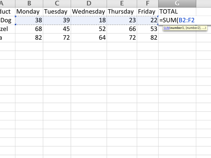
This will result in the sum of the values in the array you've selected.

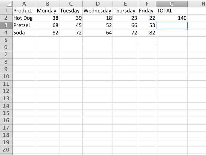
Now, we want to do that same function for the next three rows. We've got two options

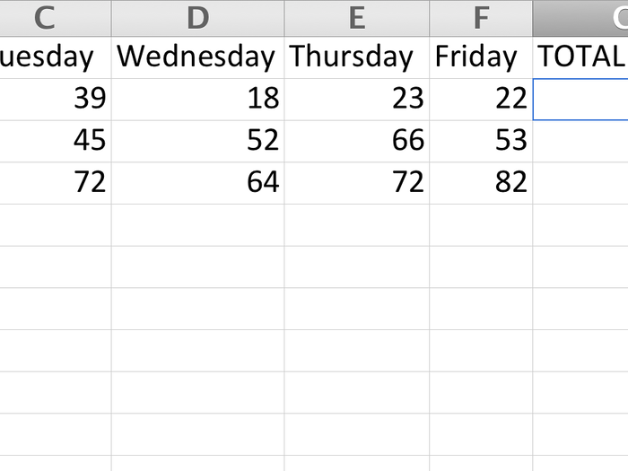
2. The first thing we could do is double click the bottom right hand corner. This will fill in the rest of the rows in the G column, provided there is data on that row in the F column.

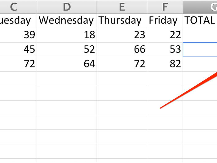
3. Alternatively, we can click and drag that down.

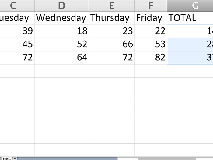
4. Now let's look at SUMPRODUCT. Let's say the business we described in the first table sold its products for different prices on different days, indicated in the second table.

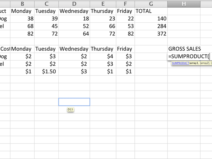
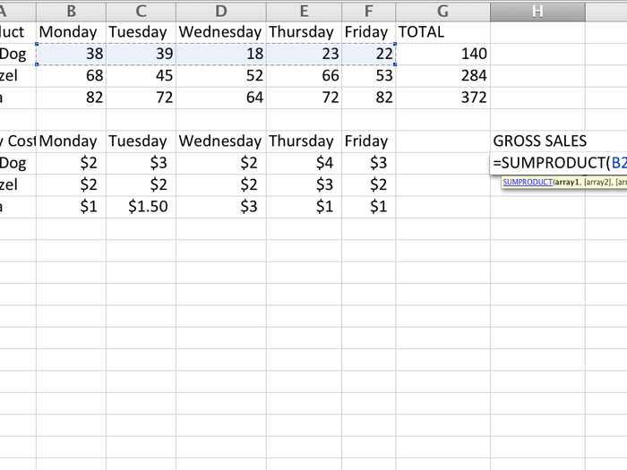
With SUMPRODUCT, we select the array of Hot Dogs from the first table.

Then we select the array of the corresponding prices from the second table.

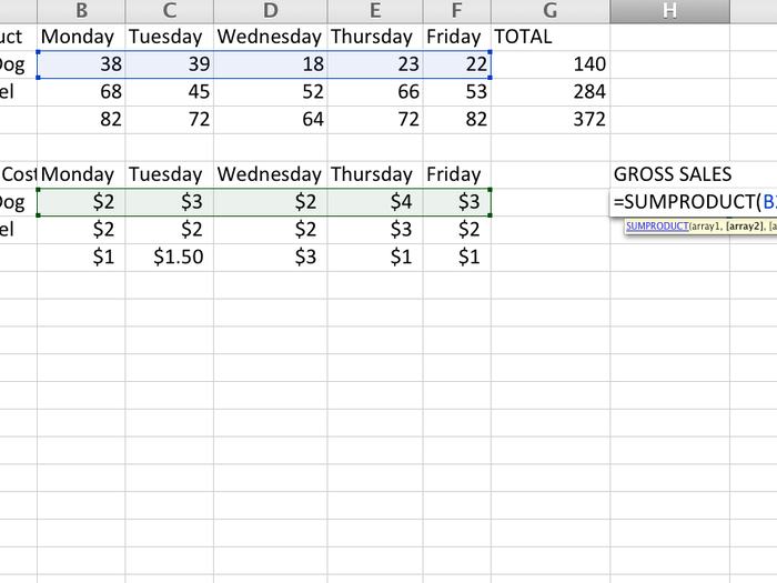
Then, we drag the function down and have our answers for how much total revenue we made.

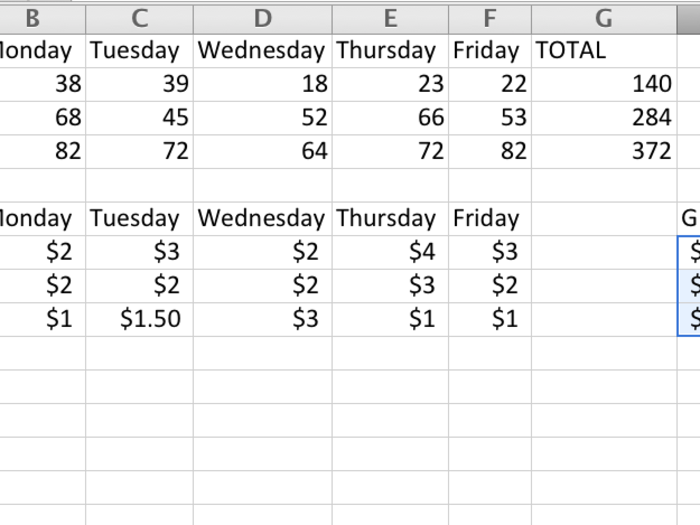
5. Let's say we want to find out the average number of items we sell on a given day. You'd use the AVERAGE formula.

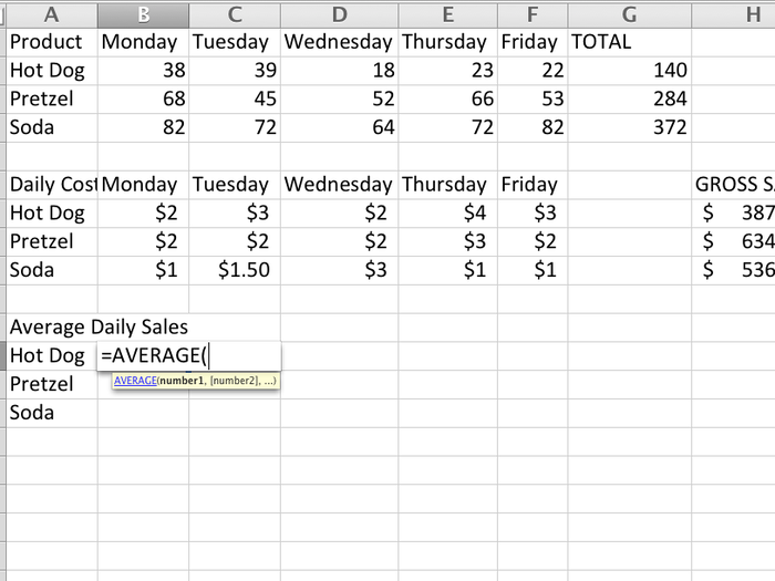
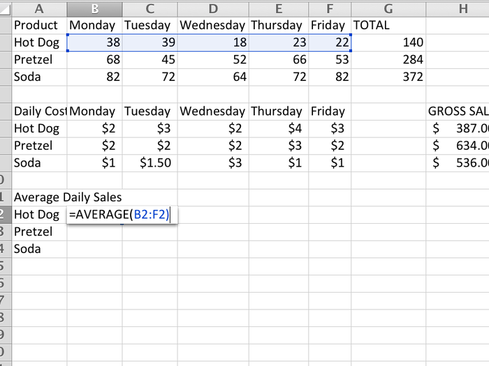
Just select the array of values that you want to average.

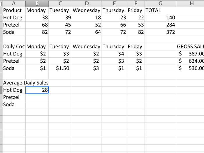
Then Excel will tell you what it is.

6. Now we're going to talk about using dollar signs in formulas. Let's try to make a simple times table. In the first cell, we type in the formula for 1 times 1.

We drag the first cell to the right, to copy the function over.

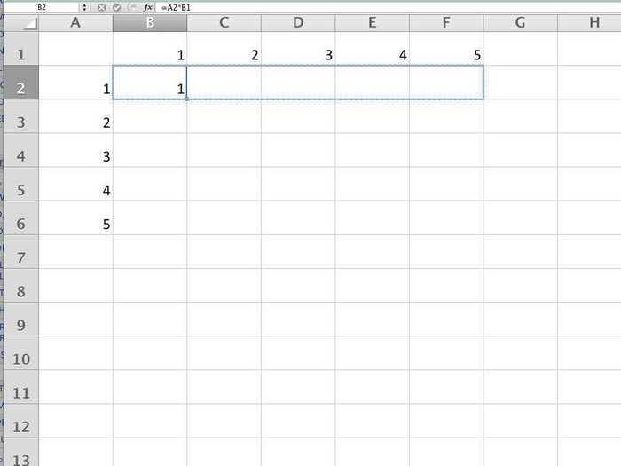
But wait, something went terribly wrong. 5 times 1 is not 120.

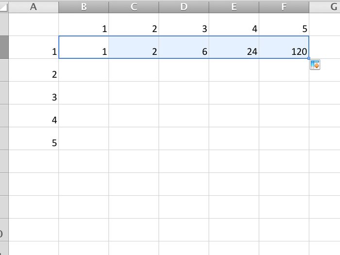
When we copied the cell over, it copied the formula over exactly as written. What we need to do is fix the original formula so that doesn't happen.

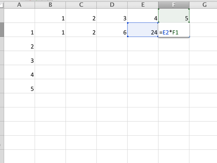
In an excel formula, a $ means an "absolute reference." By typing $A2 instead of A2, when we copy the formula it's going to lock in the value of the first multiple in Column A.

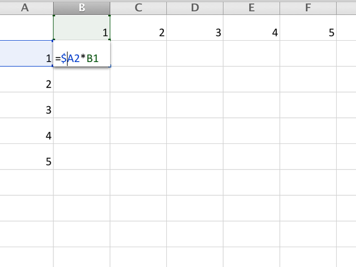
So when we copy that over it looks like this. Now let's copy this row down to fill in the rest of the table.

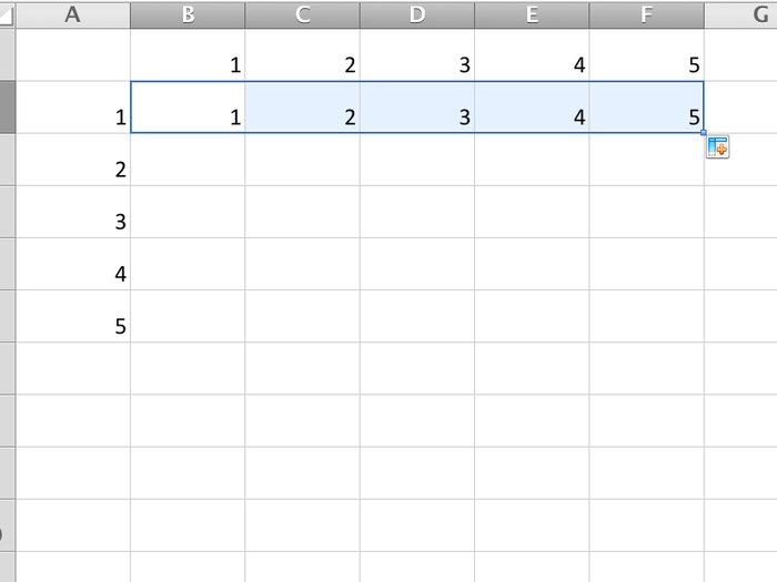
Something once again went horribly wrong.

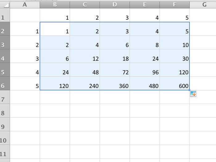
So even though the first term of each equation is locked into Column A, the second term isn't locked into Row 1. As a result, when we copied the formula down, it adjusted the position of the second term.

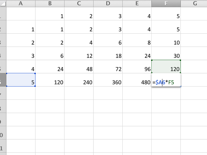
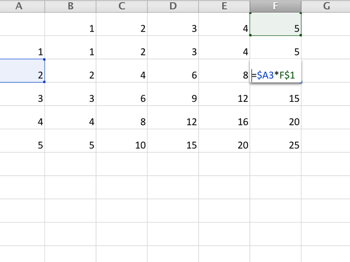
Let's fix the formula and write B$1 instead of B1. This will lock in the second term to be the relevant value on row 1.

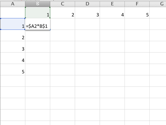
When we copy it across again we don't have any problems.

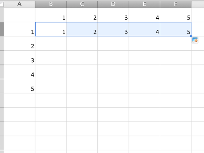
The we drag it down, and viola, by using $ we were able to lock in all the correct values. Nice.

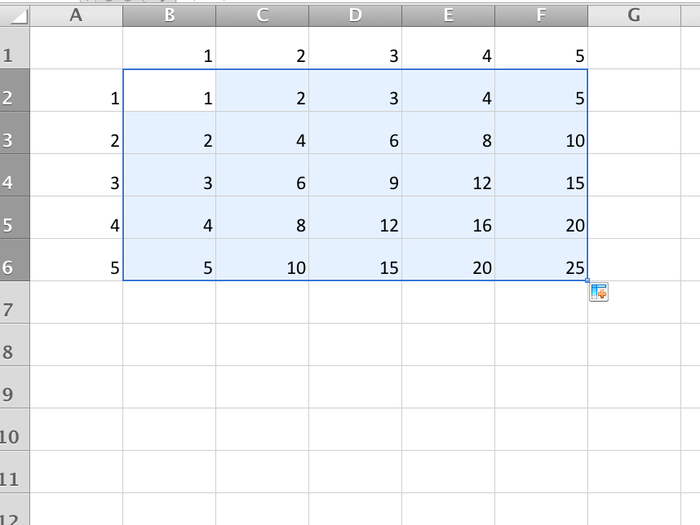
See how in the formulas of each cell, each of the column and row values that don't have a dollar sign in front of them shift with each cell, while the rows or columns with a dollar sign remain either A or 1.

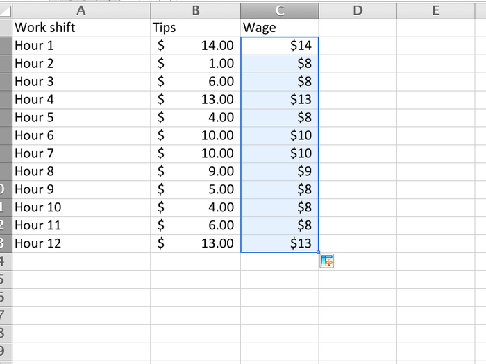
7. Let's say you wait tables for a restaurant in a state that requires you make an $8 minimum wage every hour. If you make more than $8 in tips, the restaurant doesn't pay you. If you make less, the restaurant pays you the money you need to make it to $8.

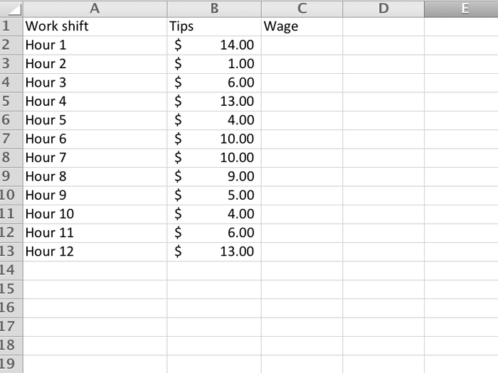
In this example, we're going to use the IF function. We're going to program it so that if the value in column B is less than $8, we replace it with $8.

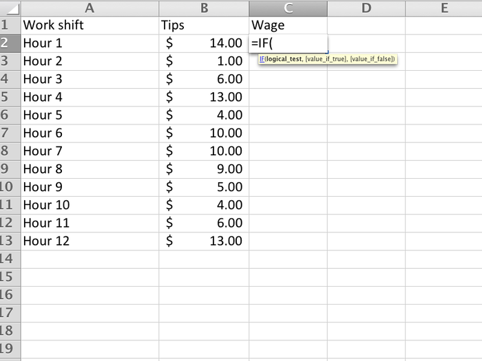
The first part of the IF function is the logical test. This will be evaluated whether it is true or false.

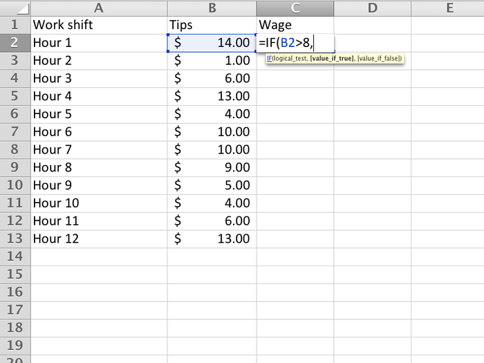
The next part tells it what to put in the cell if the logical test is true. In this case, if the value in B2 is greater than 8, we just want to put B2 in that cell.

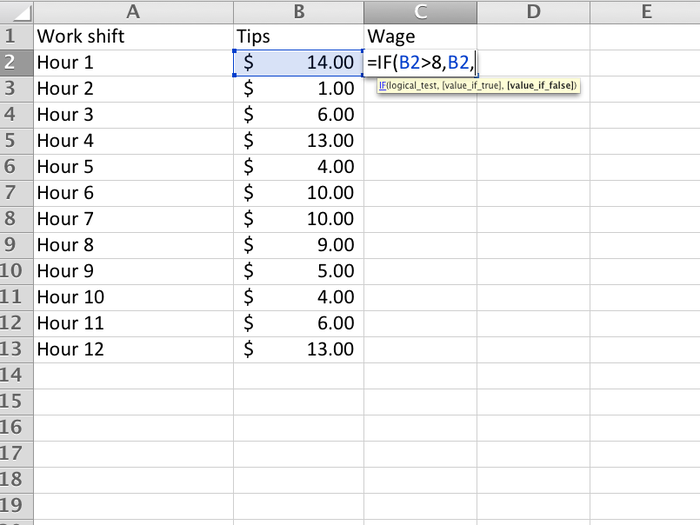
The last part is what to do if the logical test is false. If B2 is not greater than 8, then we want to make it $8.

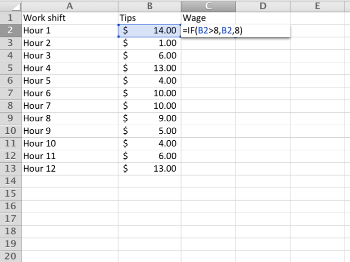
Once we fill in the whole column, you'll see how any value less than 8 has been replaced with 8, while all values greater than 8 are the same. This is a simple example of how to use the IF function.

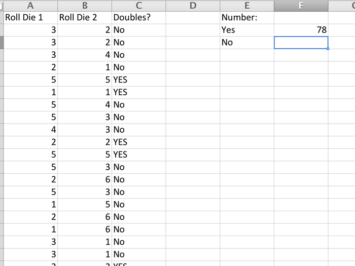
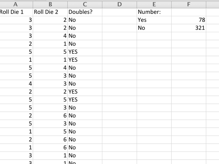
8. Let's say we run a simulation of 400 rolls of 2 dice. We then use an IF statement (in column C) to find out if they're doubles. If we want to know how many doubles there were, we can use the COUNTIF function.

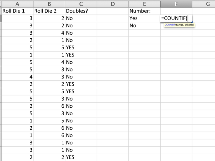
The COUNTIF function will tell you how many elements of a selected set match a given criterion. First, we select the given set of responses.

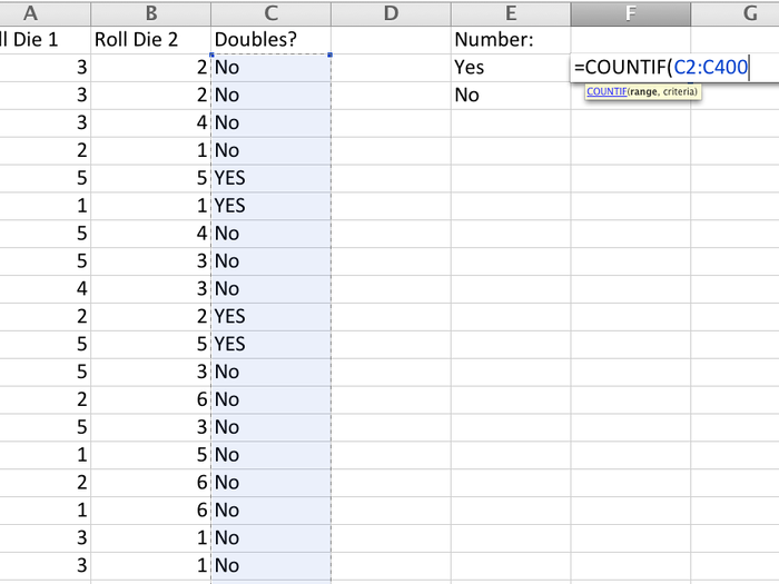
Then we tell it what we want it to count. In this case, we want to know how many times the counter finds "YES" in column C, which will tell us how many times we rolled doubles.

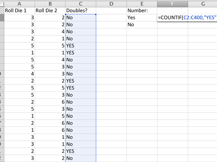
In this case, as we can see, we rolled doubles 78 times.

We can then do the same process for "No."

So you're off to a good start. Ready to move up a level?

12 Basic Shortcuts That Will Make You An Excel Guru And Add Hours To Your Life >